This page contains the
R code - Multivariate Analysis of Ecological Data
# Chapter 1: Multivariate Data in Environmental Science
# First read in the data set "bioenv" from the Excel file, call it bioenv

# For example, on Windows PC's, copy table, and then type the command:  bioenv <- read.table("clipboard")

# (Do not copy and paste the above command, otherwise you will lose the data in the clipboard!)
a <- bioenv[,1]; b <- bioenv[,2]; c <- bioenv[,3]; d <- bioenv[,4]; e <- bioenv[,5]

x <- bioenv[,6]; y <- bioenv[,7]; z <- bioenv[,8]; s <- bioenv[,9]
# make a numerical version of sediment, with order C, S, G
sed <- rep(1, length(s)); sed[s=="S"] <- 2; sed[s=="G"] <- 3
# draw three histograms and barchart, of environmental variables
par(mfrow=c(1,4))

hist(x, breaks=c(50,60,70,80,90,100), main="", xlab="Depth", ylim=c(0,12))

hist(y, breaks=c(0,2,4,6,8,10), main="", xlab="Pollution", ylim=c(0,12), ylab="")

hist(z, breaks=c(2.4,2.65,2.90,3.15,3.4,3.65), main="", xlab="Temperature", ylim=c(0,12), ylab="")

hist(sed, breaks=(c(0.5, 1, 1.5, 2, 2.5, 3, 3.5)-0.25), main="", xlab="Sediment", ylim=c(0,12), ylab="")
# draw five histograms of species abundances, with same scales on both axes
par(mfrow=c(1,5))

hist(a, breaks=c(0,5,10,15,20,25,30,35,40,45), ylim=c(0,21), main="")

hist(b, breaks=c(0,5,10,15,20,25,30,35,40,45), ylim=c(0,21), main="", ylab="")

hist(c, breaks=c(0,5,10,15,20,25,30,35,40,45), ylim=c(0,21), main="", ylab="")

hist(d, breaks=c(0,5,10,15,20,25,30,35,40,45), ylim=c(0,21), main="", ylab="")

hist(e, breaks=c(0,5,10,15,20,25,30,35,40,45), ylim=c(0,21), main="", ylab="")
# define a function panel.cor that will print the correlations in different sizes

# in the pairs function
panel.cor <- function(x, y, digits=3, prefix="", cex.cor) {

	usr <- par("usr"); on.exit(par(usr))

           par(usr = c(0, 1, 0, 1))

           r <- cor(x, y)

           txt <- format(c(r, 0.123456789), digits=digits)[1]

           txt <- paste(prefix, txt, sep="")

           if(missing(cex.cor))

           cex <- 0.8/strwidth(txt)

           if(r<0) cex<- 0.95/strwidth(txt)

           text(0.5, 0.5, txt, cex = cex * (abs(r)^2.5+0.5))

           }

env <- cbind(x,y,z)

colnames(env) <- c("Depth","Pollution","Temperature")

rownames(env) <- rownames(bioenv)

par(mfrow=c(1,1))

pairs(env,lower.panel=panel.smooth,upper.panel=panel.cor)
# code sediment into two categories, (C,S)=0 and (G)=1
sed2 <- s=="G"
# point biserial correlations between env and sed2
cor(cbind(env,sed2))[1:3,4]
      Depth   Pollution Temperature

 0.61141801 -0.52036287 -0.01453911
# EXTRA: permutation tests for point-biserials

# for example, for the first variable, depth

point_biserial <- rep(0,10000)

point_biserial[1] <- cor(cbind(env,sed2))[1,4]

set.seed(193)

for(k in 2:10000) {

  sed2.perm <- sample(sed2)

  point_biserial[k] <- cor(cbind(env,sed2.perm))[1,4]

  }

# p-value

sum(abs(point_biserial)>=abs(point_biserial[1]))/10000
[1] 0.0011
# draw three box-and-whisker plots
par(mfrow=c(1,3))

boxplot(x~as.factor(sed), ylim=c(40,100), ylab="Depth", names=c("C","S","G"))

boxplot(y~as.factor(sed), ylim=c(0,10), ylab="Pollution", names=c("C","S","G"))

boxplot(z~as.factor(sed), ylim=c(2,3.6), ylab="Temperature", names=c("C","S","G"))
# matrix of scatterplots for species abundances, with correlations in lower panel

pairs(bioenv[,1:5],upper.panel=panel.smooth,lower.panel=panel.cor)
# matrix of scatterplots with linear regression lines
bio <- bioenv[,1:5]

par(mfrow=c(5,3), mar=c(2.5,2,1,1), mgp=c(2.5,0.5,0), cex.axis=0.8)

for(i in 1:5){

  for(j in 1:3){

    plot(env[,j],bio[,i], xlab="", ylab="")

    reg<-lm(bioenv[,i]~env[,j])

    abline(reg$coefficients[1], reg$coefficients[2], lty=2, col="red")

    }

  }
# box-and-whisker plots of five species for three sediment types
par(mfrow=c(1,5), mar=c(3,4,1,1), mgp=c(2,0.7,0))

boxplot(a~as.factor(sed), ylab="a", names=c("C","S","G"))

boxplot(b~as.factor(sed), ylab="b", names=c("C","S","G"))

boxplot(c~as.factor(sed), ylab="c", names=c("C","S","G"))

boxplot(d~as.factor(sed), ylab="d", names=c("C","S","G"))

boxplot(e~as.factor(sed), ylab="e", names=c("C","S","G"))
# EXTRA: permutation test on correlation coefficient
permcor <- rep(0, 10000)

permcor[1] <- cor(x,y)

set.seed(12347)

for(iperm in 2:10000) {

  yperm <- y[sample(30)]

  permcor[iperm] <- cor(x,yperm)

  }

hist(permcor, breaks=seq(-0.7,0.7,0.05), main="", xlab="correlation", ylab="frequency")

sum(abs(permcor)>=abs(permcor[1]))
[1] 315
# Chapter 3: Measurement Scales, Transformations and Standardization
# Some Box-Cox transformations
BoxCox <- matrix(seq(0.1,30,0.1), ncol=1)

BoxCox <- cbind(BoxCox, (1/0.5) * (BoxCox[,1]^0.5-1))

BoxCox <- cbind(BoxCox, (1/0.25) * (BoxCox[,1]^0.25-1))

BoxCox <- cbind(BoxCox, (1/0.05) * (BoxCox[,1]^0.05-1))

BoxCox <- cbind(BoxCox, log(BoxCox[,1]))


par(mar=c(2,2,1,1), cex.axis=0.8, mgp=c(3,0.5,0))

plot(BoxCox[,1], BoxCox[,3], type="n", xlab="", ylab="", xlim=c(0, 30), ylim=c(-5,10), bty="n", xaxt="n", yaxt="n")

axis(1, pos=0, at=seq(0,30,5), labels=c("","5","10","15","20","25","30"))

axis(2, pos=0, at=seq(-5,10,5), labels=c("-5","0","5","10"))

lines(BoxCox[,1],BoxCox[,2], col="chocolate", lwd=2)

lines(BoxCox[,1],BoxCox[,3], col="forestgreen", lwd=2)

lines(BoxCox[,1],BoxCox[,4], col="gray", lwd=2)

lines(BoxCox[,1],BoxCox[,5], col="black", lwd=2)
# Chapter 4: Measures of Distance Between Samples: Euclidean
# ------------------------------------------------------------------------------------------------------


# means and standard deviations of the three continuous variables x=Depth, y=Polln, z=Temp
xyz <- bioenv[,6:8]

apply(xyz,2,mean)
    Depth     Polln      Temp

74.433333  4.516667  3.056667
apply(xyz,2,sd)
     Depth      Polln       Temp

15.6153844  2.1412345  0.2812329
# standardized Euclidean distances between 30 samples, based on three continuous variables

# standardization using function scale; Euclidean distances using function dist
xyzs  <- apply(bioenv[,6:8], 2, scale)

Dxyzs <- dist(xyzs)

round(Dxyzs,3)
       1     2     3     4     5    ...

2  3.681

3  2.977 1.741

4  2.708 2.980 1.523

5  1.642 2.371 1.591 2.139

.

.

.
# means and variances of the five count variables a, b, c, d, e
abcde <- bioenv[,1:5]

apply(abcde,2,mean)
        a         b         c         d         e

13.466667  8.733333  8.400000 10.900000  2.966667
apply(abcde,2,var)
        a         b         c         d         e

157.63678  83.44368  73.62759  44.43793  15.68851
# calculations of row profiles, average row profile and chi-square distances
rowpro <- abcde/apply

avepro <- apply(abcde,2,sum)/sum(apply(abcde,2,sum))

chid <- dist( rowpro%*%diag(1/sqrt(avepro)) )

round(chid, 3)
       s1    s2    s3    s4    s5   ...

s2  1.139

s3  0.855 1.137

s4  1.392 1.630 1.446

s5  1.093 0.862 1.238 2.008
.

.

.
# EXTRA: functions chidist and chidistraw for chi-square distances

# function to calculate chi-square distances between row or column profiles of a matrix

# e.g. chidist(N,1) calculates the chi-square distances between row profiles

#      (for row profiles, chidist(N) is sufficient)

#      chidist(N,2) calculates the chi-square distances between column profiles

chidist <- function(mat,rowcol=1) {

  mat <- as.matrix(mat)

  if(rowcol==1) {

    prof<-mat/apply(mat,1,sum)

    rootaveprof<-sqrt(apply(mat,2,sum)/sum(mat))

    }

  if(rowcol==2) {

    prof<-t(mat)/apply(mat,2,sum)

    rootaveprof<-sqrt(apply(mat,1,sum)/sum(mat))

    }

    dist(scale(prof,F,rootaveprof))

}

# function to calculate chi-square distances between row or column counts of a matrix (not profiles)

# e.g. chidistraw(N,1) calculates the chi-square distances between rows

#      (for rows, chidistraw(N) is sufficient)

#      chidistraw(N,2) calculates the chi-square distances between columns

chidistraw <- function(mat,rowcol=1) {

  mat <- as.matrix(mat)

  if(rowcol==1) {

    raw<-mat

    rootave<-sqrt(apply(mat,2,mean))

    }

  if(rowcol==2) {

    raw<-t(mat)

    rootave<-sqrt(apply(mat,1,mean))

    }

    dist(scale(raw,F,rootave))

}


chid    <- chidist(abcde)

chidraw <- chidistraw(abcde)
# Chapter 5: Measures of Distance Between Samples: Non-Euclidean
# Bray-Curtis dissimilarity between sites based on count data

# compute site sums, and then rescale Manhattan (city-block) distances

# by the inverses of their sums
abcde.sums <- apply(abcde, 1, sum)

n <- nrow(abcde)

BC <- dist(abcde, method="manhattan")

BC <- as.matrix(BC)/(matrix(abcde.sums, nrow=n, ncol=n) + matrix(abcde.sums, nrow=n, ncol=n, byrow=T))

BC <- as.dist(BC)

round(100*BC, 1)
       s1    s2    s3    s4    s5    ...

s2   45.7

s3   29.6  48.1

s4   46.7  55.6  46.7

s5   47.7  34.8  50.8  78.6

.

.

.
# EXTRA: function to compute Bray-Curtis dissimilarity

# function to calculate Bray-Curtis dissimilarity indices between rows

# of an abundance matrix (assuming sites are rows)

# e.g. braycurtis(N) calculates the Bray-Curtis indices between rows of N

#      (if sites are columns, say braycurtis(N,2))

braycurtis <- function(mat, rowcol=1) {

  mat <- as.matrix(mat)

  if(rowcol==1) {

    mat.sums <- apply(mat, 1, sum)

    n <- dim(mat)[1]

    BC <- dist(mat, method="manhattan")

    BC <- as.matrix(BC)/(matrix(mat.sums, nrow=n, ncol=n) + matrix(mat.sums, nrow=n, ncol=n, byrow=T))

  }

  if(rowcol==2) {

    mat.sums <- apply(mat, 1, sum)

    n <- dim(mat)[2]

    BC <- dist(t(mat), method="manhattan")

    BC <- as.matrix(BC)/(matrix(mat.sums, nrow=n, ncol=n) + matrix(mat.sums, nrow=n, ncol=n, byrow=T))

  }

  as.dist(BC)

}

round(100*braycurtis(abcde), 1)
       s1    s2    s3    s4    s5   ...

s2   45.7

s3   29.6  48.1

s4   46.7  55.6  46.7

s5   47.7  34.8  50.8  78.6

.

.

.
|
# Bray-Curtis on relativized data
BCrel <- 100*braycurtis(abcde/apply(abcde, 1, sum))

round(BCrel, 1)
       s1    s2    s3    s4    s5    ...

s2   48.1

s3   29.6  48.1

s4   50.0  59.3  50.0

s5   51.0  30.1  52.6  75.4

.

.

.
# graphical comparison of chi-square and Bray-Curtis for raw and relative counts (profiles)
par(mfrow=c(1,2), cex.axis=0.8, mar=c(4.2,4,2,2))

plot(100*BC, chidraw, col="forestgreen", cex=0.8, xlab="B-C raw", ylab="chi2 raw")

plot(100*BCrel, chid, col="forestgreen", cex=0.8, xlab="B-C rel", ylab="chi2 rel")
# Read in the presence/absence data from the Excel file, call it pres.abs

# For example, in Windows, copy the file, including row and column names

# (and the blank cell in top left corner), and then execute the following:
pres.abs <- read.table("clipboard")
# compute Jaccard dissimilarities between rows
pres.abs <- as.matrix(pres.abs)

jacc <- 1 - (pres.abs %*% t(pres.abs) / (pres.abs %*% t(pres.abs) +pres.abs %*% t(1-pres.abs) + (1-pres.abs) %*% t(pres.abs)))

round(jacc, 3)
      A     B     C     D     E     F     G

A 0.000 0.500 0.429 1.000 0.250 0.625 0.375

B 0.500 0.000 0.714 0.833 0.667 0.200 0.778

C 0.429 0.714 0.000 1.000 0.429 0.667 0.333

D 1.000 0.833 1.000 0.000 1.000 0.800 0.857

E 0.250 0.667 0.429 1.000 0.000 0.778 0.375

F 0.625 0.200 0.667 0.800 0.778 0.000 0.750

G 0.375 0.778 0.333 0.857 0.375 0.750 0.000
# EXTRA: function to compute Jaccard dissimilarities

# function to calculate Jaccard dissimilarity indices between rows

# of a presence-absence (assuming sites are rows)

# e.g. jaccard(N) calculates the Jaccard indices between rows

#      (for indices between columns, say jaccard(N,2))

jaccard <- function(PA,rowcol=1) {

  PA <- as.matrix(PA)

  if(rowcol==1) {

    jac <- 1 - (PA %*% t(PA) / (PA %*% t(PA) + PA %*% t(1-PA) + (1-PA) %*% t(PA)))

  }


  if(rowcol==2) {

    jac <- 1 - (t(PA) %*% PA / (t(PA) %*% PA + t(PA) %*% (1-PA) + t(1-PA) %*% PA))

  }

  as.dist(jac)

}

round(jaccard(pres.abs), 3)
      A     B     C     D     E     F

B 0.500

C 0.429 0.714

D 1.000 0.833 1.000

E 0.250 0.667 0.429 1.000

F 0.625 0.200 0.667 0.800 0.778

G 0.375 0.778 0.333 0.857 0.375 0.750
# standardized Euclidean distances between 30 samples, based on three continuous variables

# standardization using function scale; Euclidean distances using function dist
xyzs  <- apply(bioenv[,6:8], 2, scale)

Dxyzs <- dist(xyzs)

round(Dxyzs,3)
       1     2     3     4     5    ...

2  3.681

3  2.977 1.741

4  2.708 2.980 1.523

5  1.642 2.371 1.591 2.139

.

.

.
# means and variances of the five count variables a, b, c, d, e
abcde <- bioenv[,1:5]

apply(abcde,2,mean)
        a         b         c         d         e

13.466667  8.733333  8.400000 10.900000  2.966667
apply(abcde,2,var)
        a         b         c         d         e

157.63678  83.44368  73.62759  44.43793  15.68851
# calculations of row profiles, average row profile and chi-square distances
rowpro<-abcde/apply

avepro<-apply(abcde,2,sum)/sum(apply(abcde,2,sum))

chid<-dist( rowpro%*%diag(1/sqrt(avepro)) )

round(chid, 3)
       s1    s2    s3    s4    s5   ...

s2  1.139

s3  0.855 1.137

s4  1.392 1.630 1.446

s5  1.093 0.862 1.238 2.008
.

.

.
# EXTRA: functions chidist and chidistraw for chi-square distances

# function to calculate chi-square distances between row or column profiles of a matrix

# e.g. chidist(N,1) calculates the chi-square distances between row profiles

#      (for row profiles, chidist(N) is sufficient)

#      chidist(N,2) calculates the chi-square distances between column profiles

chidist <- function(mat,rowcol=1) {

  mat <- as.matrix(mat)

  if(rowcol==1) {

    prof<-mat/apply(mat,1,sum)

    rootaveprof<-sqrt(apply(mat,2,sum)/sum(mat))

    }

  if(rowcol==2) {

    prof<-t(mat)/apply(mat,2,sum)

    rootaveprof<-sqrt(apply(mat,1,sum)/sum(mat))

    }

    dist(scale(prof,F,rootaveprof))

}

# function to calculate chi-square distances between row or column counts of a matrix (not profiles)

# e.g. chidistraw(N,1) calculates the chi-square distances between rows

#      (for rows, chidistraw(N) is sufficient)

#      chidistraw(N,2) calculates the chi-square distances between columns

chidistraw <- function(mat,rowcol=1) {

  mat <- as.matrix(mat)

  if(rowcol==1) {

    raw<-mat

    rootave<-sqrt(apply(mat,2,mean))

    }

  if(rowcol==2) {

    raw<-t(mat)

    rootave<-sqrt(apply(mat,1,mean))

    }

    dist(scale(raw,F,rootave))

}

chid    <- chidist(abcde)

chidraw <- chidistraw(abcde)
# Chapter 6: Measures of Distance and Correlation Between Variables
# Distances between continuous variables
round(cor(env[,1:3]),4)
             Depth Pollution Temperature

Depth        1.0000   -0.3955     -0.0034

Pollution   -0.3955    1.0000     -0.0921

Temperature -0.0034   -0.0921      1.0000
env.rank <- apply(env[,1:3],2,rank)

env.rank[1:5,]
   Depth Pollution Temperature

1   14.0      20.0        28.5

2   17.0       8.5         1.5

3    6.5      22.0         3.0

4   10.5      28.0         8.5

5    8.5      13.5        20.0
round(cor(apply(env[,1:3],2,rank)),4)
              Depth Pollution Temperature

Depth        1.0000   -0.4233     -0.0051

Pollution   -0.4233    1.0000     -0.0525

Temperature -0.0051   -0.0525      1.0000
round(sqrt(2-2*cor(env[,1:3])),4)
             Depth Pollution Temperature

Depth       0.0000    1.6706      1.4166

Pollution   1.6706    0.0000      1.4779

Temperature 1.4166    1.4779      0.0000
round(sqrt(2-2*cor( apply(env[,1:3],2,rank ))),4)
             Depth Pollution Temperature

Depth       0.0000    1.6872      1.4178

Pollution   1.6872    0.0000      1.4509

Temperature 1.4178    1.4509      0.0000
# chi-square distance and Bray-Curtis dissimilarity between five species

# both based on their relative proportions across the sites

# using functions chidist and braycurtis defined previously

# chidist computes column profiles automatically

# for braycurtis, profiles need to be computed, in this case using scale function
chidist(abcde, 2)
          a         b         c         d

b 0.8018198

c 1.5217292 1.4065684

d 0.8701050 0.8283417 1.1574670

e 1.4058584 1.5504877 1.8548764 1.4299704
100*braycurtis(scale(abcde, center=F, scale=apply(abcde, 2, sum)), 2)
         a        b        c        d

b 28.57494

c 60.85573 56.40070

d 32.88597 33.46056 41.44459

e 53.30960 57.59499 70.38077 55.61626
# measures of association for cross-table: chi-square, phi-square and Cramer's V
crosstab <- matrix(c(6,5,0,3,5,1,2,1,7), nrow=3, byrow=T)

chisquare <- as.numeric(chisq.test(crosstab)$statistic)

chisquare/sum(crosstab)
[1] 0.51941
sqrt((chisquare/sum(crosstab))/min(nrow(crosstab)-1, ncol(crosstab)-1))
[1] 0.5096126
# chi-square distances between categories
chidist(crosstab, 2)
         1        2

2 0.396895

3 1.525014 1.664296
# parametric t-test for correlation coefficient between depth and pollution
cor.test(x,y)
        Pearson's product-moment correlation

data:  x and y

t = -2.2787, df = 28, p-value = 0.03051

alternative hypothesis: true correlation is not equal to 0

95 percent confidence interval:

 -0.66152649 -0.04110943

sample estimates:

       cor

-0.3955208
# permutation test for correlation coefficient

# note that this run gives the p-value of 0.0315

# reported in Chapter 1.  Running this code without

# setting the seed gives a different set of random

# permutations and thus a slightly different estimate

# of the p-value.
permcor <- rep(0, 10000)

permcor[1] <- cor(x,y)

set.seed(12347)

for(iperm in 2:10000) {

  permcor[iperm] <- cor(x,sample(y))

  }

par(mfrow=c(1,1))

hist(permcor, breaks=seq(-0.7,0.7,0.05), main="", xlab="correlation", ylab="frequency")

sum(abs(permcor)>=abs(permcor[1]))/10000
[1] 0.0315
# Chapter 7: Hierarchical Cluster Analysis
# hierarchical clustering of Jaccard dissimilarities, complete linkage

# default dendrogram, then dendrogram with branches down to 0
jacc.clus <- hclust(jaccard(pres.abs))

plot(jacc.clus)

plot(jacc.clus, hang=-1, main="Clustering of Jaccard dissimilarities", xlab="")
# cutting the tree to form 3 groups (group numbers 1 and 2 interchanged compared Chap. 7)
cutree (jacc.clus, 3)
A B C D E F G

1 2 1 3 1 2 1
# clustering the dissimilarities between species, first by 1-correlation, then by Jaccard

# (in Exhibit 7.9, the level is reversed in terms of similarity: correlation, and 1-Jaccard
plot(hclust(as.dist(1-cor(pres.abs))))

plot(hclust(jaccard(t(pres.abs))))
# clustering of 30 sites in terms of their Euclidean distances on depth, pollution, temperature

# distance matrix Dxyzs computed in Chapter 4
plot(hclust(Dxyzs), labels=rownames(bioenv), xlab="sites")
# cut tree into 4 clusters
cutree(hclust(Dxyzs), 4)
[1] 1 2 1 3 1 4 1 1 1 3 1 2 3 2 2 2 2 1 4 1 1 1 2 1 2 4 2 4 1 2
###### TO BE CONTINUED ######
R code - Biplots in Practice
# Chapter 1: Biplots - the basic idea
# Read in European indicators data set (Exhibit 1.1) into data frame EU2008 (see p.168)

# For example, on Windows PC's, copy table, and then type the command:  EU2008 <- read.table("clipboard")

# (Do not copy and paste the above command, otherwise you will lose the data in the clipboard!)
windows(width = 11, height = 6)

par(mfrow = c(1,2))

plot(EU2008[,2:1], type = "n", cex.axis = 0.7, xlab = "GDP/capita", ylab = "Purchasing power/capita")

text(EU2008[,2:1], labels = rownames(EU2008), col = "forestgreen", font = 2)

plot(EU2008[,2:3], type = "n", cex.axis = 0.7, xlab = "GDP/capita", ylab = "Inflation rate")

text(EU2008[,2:3], labels = rownames(EU2008), col = "forestgreen", font = 2)
# Note: we use "forestgreen" for the labels above, more like the green in the book.

# Install the R package rgl for 3-d graphics, and then load as follows:
library(rgl)

plot3d(EU2008[,c(2,1,3)], xlab = "GDP", ylab = "Purchasing power", zlab = "Inflation", font = 2, col = "brown", type = "n")

text3d(EU2008[,c(2,1,3)], text = rownames(EU2008), font = 2, col = "forestgreen")
# Chapter 2: Regression biplots
# 'bioenv' data set with 8 columns (first 8 columns of Exhibit 2.1) in data frame bioenv. d is species d, y is pollution, x is depth
d <- bioenv[,4]

y <- bioenv[,6]

x <- bioenv[,7]


summary(lm(d ~ y + x))
Call:

lm(formula = d ~ y + x)


Residuals:

     Min       1Q   Median       3Q      Max

-11.7001  -2.4684   0.1749   3.0563   9.1803


Coefficients:

            Estimate Std. Error t value Pr(>|t|)

(Intercept)  6.13518    6.25721   0.980  0.33554

y           -1.38766    0.48745  -2.847  0.00834 **

x            0.14822    0.06684   2.217  0.03520 *

---

Signif. codes:  0 '***' 0.001 '**' 0.01 '*' 0.05 '.' 0.1 ' ' 1


Residual standard error: 5.162 on 27 degrees of freedom

Multiple R-squared: 0.4416,     Adjusted R-squared: 0.4003

F-statistic: 10.68 on 2 and 27 DF,  p-value: 0.0003831
# Two ways of calculating regression coefficients

# 1. by doing the regression on standardized variables
ds <- (d-mean(d)) / sd(d)

ys <- (y-mean(y)) / sd(y)

xs <- (x-mean(x)) / sd(x)

summary(lm(ds ~ ys + xs))
Call:

lm(formula = ds ~ ys + xs)


Residuals:

     Min       1Q   Median       3Q      Max

-1.75515 -0.37028  0.02623  0.45847  1.37715


Coefficients:

              Estimate Std. Error  t value Pr(>|t|)

(Intercept)  2.487e-17  1.414e-01 1.76e-16  1.00000

ys          -4.457e-01  1.566e-01   -2.847  0.00834 **

xs           3.472e-01  1.566e-01    2.217  0.03520 *


---

Signif. codes:  0 '***' 0.001 '**' 0.01 '*' 0.05 '.' 0.1 ' ' 1


Residual standard error: 0.7744 on 27 degrees of freedom

Multiple R-squared: 0.4416,     Adjusted R-squared: 0.4003

F-statistic: 10.68 on 2 and 27 DF,  p-value: 0.0003831
# 2. by direct calculation
lm(d ~ y + x)$coefficients[2] * sd(y) / sd(d)
         y

-0.4457286
lm(d ~ y + x)$coefficients[3] * sd(x) / sd(d)
        x

0.3471993
# Finding and storing the standardized regression coefficients for all five species - matrix B in (2.2)
B <- lm(bioenv[,1] ~ y+x)$coefficients[2:3] * c(sd(y),sd(x)) / sd(bioenv[,1])

for(j in 2:5) B <- rbind(B,lm(bioenv[,j] ~ y + x)$coefficients[2:3] * c(sd(y),sd(x)) / sd(bioenv[j]))


B
           y           x

B -0.7171713  0.02465266

  -0.4986038  0.22885450

   0.4910580  0.07424574

  -0.4457286  0.34719935

  -0.4750841 -0.39952072
# EXTRA: storing the variance explained for each regression


var.expl <- var(lm(bioenv[,1] ~ y + x)$fitted.values)

for(j in 2:5) var.expl <- var.expl + var(lm(bioenv[,j] ~ y + x)$fitted.values)


for(j in 1:5) print(var(lm(bioenv[,j] ~ y + x)$fitted.values) / var(bioenv[,j]))
[1] 0.5289281

[1] 0.3912441

[1] 0.2178098

[1] 0.4416404

[1] 0.2351773
# EXTRA: overall variance explained for all 5 species


var.expl / sum(apply(bioenv[,1:5], 2, var))
[1] 0.4145226
# EXTRA: doing the same as previous 'EXTRA', but for three predictor variables, adding z = temperature


z <- bioenv[,8]

var.expl3 <- var(lm(bioenv[,1] ~ y + x + z)$fitted.values)

for(j in 2:5) var.expl3 <- var.expl3 + var(lm(bioenv[,j] ~ y + x + z)$fitted.values)


for(j in 1:5) print(var(lm(bioenv[,j] ~ y + x + z)$fitted.values) / var(bioenv[,j]))
[1] 0.5569366

[1] 0.3924837

[1] 0.2181056

[1] 0.4416436

[1] 0.2463643
var.expl3 / sum(apply(bioenv[,1:5], 2, var))
[1] 0.4271042
# Drawing a regression biplot (Exhibit 2.5) using standardized values of x and y.

# Species labels are put at the point, arrows are 5% shorter

# Note: either close the previous graphics window, or open a new one

# - on Windows machines open with command win.graph()
win.graph()

plot(xs, ys, xlab = "x*(depth)", ylab = "y*(pollution)", type = "n", asp = 1, cex.axis = 0.7)

text(xs, ys, labels = rownames(bioenv), col = "forestgreen")

text(B[,2:1], labels = colnames(bioenv[,1:5]), col = "chocolate", font = 4)

arrows(0, 0, 0.95*B[,2], 0.95*B[,1], col = "chocolate", angle = 15, length = 0.1)
# (Notice again that we have varied the color definitions to be more like those in the book)
# Chapter 3: Generalized linear model biplots
# d0 is the fourth-root transformed d; do regression of d0 on ys and xs
d0 <- d^0.25

summary(lm(d0 ~ ys + xs))
Call:

lm(formula = d0 ~ ys + xs)


Residuals:

     Min       1Q   Median       3Q      Max

-1.50933 -0.04458  0.13950  0.25483  0.85149


Coefficients:

            Estimate Std. Error t value Pr(>|t|)

(Intercept)  1.63908    0.09686  16.923 6.71e-16 ***

ys          -0.28810    0.10726  -2.686   0.0122 *

xs           0.05959    0.10726   0.556   0.5831

---

Signif. codes:  0 '***' 0.001 '**' 0.01 '*' 0.05 '.' 0.1 ' ' 1


Residual standard error: 0.5305 on 27 degrees of freedom

Multiple R-squared: 0.2765,     Adjusted R-squared: 0.2229

F-statistic: 5.159 on 2 and 27 DF,  p-value: 0.01266
# EXTRA: saving all the coefficients for the double square-root regressions (Exhibit 3.1).

# We also accumulate the variance explained in each and compute overall variance explained


dsqrt_abcde       <- bioenv[,1:5]^0.25

dsqrt_abcde_coefs <- lm(dsqrt_abcde[,1] ~ ys + xs)$coefficients

dsqrt.var.expl    <- var(lm(dsqrt_abcde[,1] ~ ys + xs)$fitted.values)


for(j in 2:5){

  dsqrt_abcde_coefs <- rbind(dsqrt_abcde_coefs, lm(dsqrt_abcde[,j] ~ ys + xs)$coefficients)

  dsqrt.var.expl <- dsqrt.var.expl + var(lm(dsqrt_abcde[,j] ~ ys + xs)$fitted.values)

  }


for(j in 1:5) print(var(lm(dsqrt_abcde[,j] ~ ys + xs)$fitted.values) / var(dsqrt_abcde[,j]))
[1] 0.6052581

[1] 0.3621872

[1] 0.1591791

[1] 0.2764936

[1] 0.2284871
dsqrt.var.expl / sum(apply(dsqrt_abcde[,1:5], 2, var))
[1] 0.3393836
# EXTRA: drawing the biplot of Exhibit 3.2


plot(xs, ys, xlab = "x*(depth)", ylab = "y*(pollution)", type = "n", asp = 1, cex.axis = 0.7)

text(xs, ys, labels = rownames(bioenv), col = "forestgreen")

text(dsqrt_abcde_coefs[,3:2], labels = colnames(bioenv[,1:5]), col = "chocolate", font = 4)

for(j in 1:5) arrows(0, 0, 0.95*dsqrt_abcde_coefs[j,3], 0.95*dsqrt_abcde_coefs[j,2], col = "chocolate", angle = 15, length = 0.1)
# Performing Poisson regression for species d:
summary(glm(d ~ ys + xs, family = poisson))
Call:

glm(formula = d ~ ys + xs, family = poisson)


Deviance Residuals:

    Min       1Q   Median       3Q      Max

-4.4123  -0.7585   0.1637   0.8262   2.7565


Coefficients:

            Estimate Std. Error z value Pr(>|z|)

(Intercept)  2.29617    0.06068  37.838  < 2e-16 ***

ys          -0.33682    0.07357  -4.578 4.69e-06 ***

xs           0.19963    0.06278   3.180  0.00147 **

---

Signif. codes:  0 '***' 0.001 '**' 0.01 '*' 0.05 '.' 0.1 ' ' 1


(Dispersion parameter for poisson family taken to be 1)


    Null deviance: 144.450  on 29  degrees of freedom

Residual deviance:  88.671  on 27  degrees of freedom

AIC: 208.55


Number of Fisher Scoring iterations: 5
# To get error deviance for Poisson regression of species d:
poisson.glm <- glm(d~ys+xs, family=poisson)

poisson.glm$deviance/poisson.glm$null.deviance
[1] 0.6138564
# EXTRA: saving all the coefficients for the Poisson regressions (Exhibit 3.4)


abcde <- bioenv[,1:5]

pois_abcde_coefs <- glm(abcde[,1] ~ ys + xs, family = poisson)$coefficients

for(j in 2:5) pois_abcde_coefs <- rbind(pois_abcde_coefs, glm(abcde[,j] ~ ys + xs, family=poisson)$coefficients)


pois_abcde_coefs
                 (Intercept)         ys          xs

pois_abcde_coefs   2.1786692 -1.1254080 -0.06714289

                   1.8525985 -0.8122742  0.18286062

                   2.0411089  0.4174381  0.05321664

                   2.2961652 -0.3368244  0.19963421

                   0.8277491 -0.8234332 -0.56805285
# Performing logistic regression for species d, after converting to presence/absence:
d01 <- d > 0

summary(glm(d01 ~ ys + xs, family = binomial))
Call:

glm(formula = d01 ~ ys + xs, family = binomial)


Deviance Residuals:

    Min       1Q   Median       3Q      Max

-2.2749   0.2139   0.2913   0.3884   1.2874


Coefficients:

            Estimate Std. Error z value Pr(>|z|)

(Intercept)   2.7124     0.8533   3.179  0.00148 **

ys           -1.1773     0.6522  -1.805  0.07105 .

xs           -0.1369     0.7097  -0.193  0.84708

---

Signif. codes:  0 '***' 0.001 '**' 0.01 '*' 0.05 '.' 0.1 ' ' 1


(Dispersion parameter for binomial family taken to be 1)


    Null deviance: 19.505  on 29  degrees of freedom

Residual deviance: 15.563  on 27  degrees of freedom

AIC: 21.563


Number of Fisher Scoring iterations: 6
# To get error deviance for logistic regression of species d:
logistic.glm <- glm(d01 ~ ys + xs, family = binomial)

logistic.glm$deviance / logistic.glm$null.deviance
[1] 0.7979165
# EXTRA: saving all the coefficients for the logistic regressions (Exhibit 3.5)


abcde01 <- abcde > 0

logit_abcde_coefs <- glm(abcde01[,1] ~ ys + xs, family = binomial)$coefficients

for(j in 2:5) logit_abcde_coefs <- rbind(logit_abcde_coefs, glm(abcde01[,j] ~ ys + xs, family = binomial)$coefficients)


logit_abcde_coefs
                  (Intercept)         ys         xs

logit_abcde_coefs   2.3842273 -2.8885410  0.8631339

                    1.2731575 -1.4183387 -0.1431720

                    0.8309807  0.9726882  0.3148828

                    2.7124406 -1.1772989 -0.1368686

                    0.2532229 -1.2796484 -0.7858995
# EXTRA: another example of a plot (Example 3.6)

# This time the arrows are drawn to the exact point and labels are offset


plot(xs, ys, type = "n", xlab = "x* (depth)", ylab = "y* (pollution)", ylim = c(-3,2.6), cex.axis = 0.7, asp = 1)

text(xs, ys, labels = rownames(bioenv), col = "forestgreen", cex=0.8)

arrows(0, 0, logit_abcde_coefs[,3], logit_abcde_coefs[,2], col = "chocolate", length = 0.1, angle = 15, lwd = 1)

text(1.05*logit_abcde_coefs[,3:2], labels = colnames(bioenv[,1:5]), col = "chocolate", font = 4, cex = 1.1)
# Chapter 4: Multidimensional scaling biplots
# 'countries' data set -- dissimilarities between 13 countries (Exhibit 4.1) -- assumed to have been read into data frame MT_matrix

# R function cmdscale performs classical multidimensional scaling

# Exhibit 4.2 is obtained as follows
plot(cmdscale(MT_matrix), type = "n", xlab = "dim 1", ylab = "dim 2", asp = 1)

text(cmdscale(MT_matrix), labels = colnames(MT_matrix), col = "forestgreen")
# EXTRA (*only* for MDS experts -- there is a bug in the cmdscale function... read on...)


# Here are the first 12 eigenvalues of the MDS (notice that warnings are given that some are negative):


cmdscale(MT_matrix, eig = TRUE, k = 12)$eig


# Function cmdscale does not allow obtaining the last (13th) eigenvalue, and there is thus a bug

# in the computation of the goodness-of-fit (GOF), which doesn't take the last dimension into account


cmdscale(MT_matrix, eig = TRUE)$GOF
[1] 0.6177913 0.6500204
# In the above the first reported GOF value is wrong. It is based on the first 12 eigenvalues only:


sum(abs(cmdscale(MT_matrix, eig = TRUE, k = 12)$eig))
[1] 264.5464
# Since it is not possible to set the number of eigenvalues to 13, we use an indirect route.

# Here is the correct total, which includes the last (negative) eigenvalue (absolute values of eigenvalues are summed)

# (the option x.ret = TRUE returns the double-centred dissimilarity matrix, -1/2 times the double-centred matrix

#  is subject to an eigenvalue decomposition to get the full set of eigenvalues and thus the correct total variance of the matrix)


MT_sum <- sum(abs(eigen(-0.5*cmdscale(MT_matrix, eig = TRUE, x.ret = TRUE)$x)$values))

MT_sum
[1] 288.0903
# The following verifies the second GOF value, which is based on the positive eigenvalues (first 8)

# (0.6500204 = 0.3821252 + 0.2678952)                 [Note: ignore the warnings again!]


cmdscale(MT_matrix, eig = TRUE, k = 12)$eig[1:2] / sum(cmdscale(MT_matrix, eig = TRUE, k = 12)$eig[1:8])
[1] 0.3821252 0.2678952
# and the following revised calculation for the first GOF value gives what the first two proportions of variance

# should have been, based on the sum of the absolute values of all 13 eigenvalues, 0.5673029 and not 0.6177913

# (0.5673029 = 0.3334984+0.2338045)


cmdscale(MT_matrix, eig = TRUE, k = 12)$eig[1:2] / MT_sum
[1] 0.3334984 0.2338045
sum(cmdscale(MT_matrix, eig = TRUE, k = 12)$eig[1:2] / MT_sum)
[1] 0.5673029
# 'atributes' data set -- country ratings on 6 attributes (Exhibit 4.3) -- assumed to have been read into data frame MT_ratings

# keep coordinates of MDS plot in MT_dims
MT_dims <- cmdscale(MT_matrix, eig = TRUE, k = 2)$points

colnames(MT_dims) <- c("dim1","dim2")
# calculate the regression coefficients of the 6 attributes on the coordinates (Exhibit 4.4)
MT_coefs <- lm(MT_ratings[,1] ~ MT_dims[,1] + MT_dims[,2])$coefficients

for(j in 2:6) MT_coefs <- rbind(MT_coefs, lm(MT_ratings[,j] ~ MT_dims[,1] + MT_dims[,2])$coefficients)
# plot the regression coefficients on the MDS plot (Exhibit 4.5)
plot(cmdscale(MT_matrix), type = "n", xlab = "dim 1", ylab = "dim 2", asp = 1)

text(cmdscale(MT_matrix), labels = colnames(MT_matrix), col = "forestgreen")

arrows(0, 0, MT_coefs[,2], MT_coefs[,3], col = "chocolate", length = 0.1, angle = 10)

text(1.2*MT_coefs[,2:3], labels = colnames(MT_ratings), col = "chocolate", font = 4, cex = 0.8)
# Function to calculate chi-square distances between row or column profiles of a matrix

# Usage: chidist(N,1) calculates the chi-square distances between row profiles (for row profiles, chidist(N) is sufficient)

#        chidist(N,2) calculates the chi-square distances between column profiles
chidist <- function(mat, rowcol = 1) {

  if(rowcol == 1) {

    prof <- mat / apply(mat, 1, sum)

    rootaveprof <- sqrt(apply(mat, 2, sum) / sum(mat))

    }

  if(rowcol == 2) {

    prof <- t(mat) / apply(mat, 2, sum)

    rootaveprof <- sqrt(apply(mat, 1, sum) / sum(mat))

    }

  dist(scale(prof, FALSE, rootaveprof))

  }
# Note: functions defined in this way are added as objects to your workspace, and are saved if the workspace is saved,

# otherwise they are lost.


# Compute chi-square distances between row profiles, perform classical MDS and plot
abcde <- bioenv[,1:5]

abcde_mds <- cmdscale(chidist(abcde), eig = TRUE, k = 4)

100 * abcde_mds$eig / sum(abcde_mds$eig)
[1] 52.364447 22.014980 16.187784 9.432789
plot(abcde_mds$points[,1:2], type = "n", xlab = "dim 1", ylab = "dim 2", xlim = c(-1.2,1.6), ylim = c(-1.1,1.8), asp = 1)

text(abcde_mds$points[,1:2], labels = rownames(abcde), col = "forestgreen")
# Now add columns (species) as biplot vectors

# First convert to row profiles and standardize in the chi-squared way
abcde_prof <- abcde / apply(abcde, 1, sum)

abcde_prof_stand <- t(t(abcde_prof) / sqrt(apply(abcde, 2, sum) / sum(abcde)))
# Perform regressions and save coefficients for plotting
mds_coefs <- lm(abcde_prof_stand[,1] ~ abcde_mds$points[,1] + abcde_mds$points[,2])$coefficients

for(j in 2:5) {

  mds_coefs <- rbind(mds_coefs, MT_coefs <- lm(abcde_prof_stand[,j] ~ abcde_mds$points[,1] + abcde_mds$points[,2])$coefficients)

  }

arrows(0, 0, mds_coefs[,2], mds_coefs[,3], col = "chocolate", length = 0.1, angle = 10)

text(1.1*mds_coefs[,2:3], labels = colnames(abcde), col = "chocolate", font = 4, cex = 0.9)
# Assume that the sediment vector has been read into a character vector; e.g., in Windows, copy the vector from the Excel file

# bioenv.xls, without the column label, and then type in the command:  sediment <- scan("clipboard", what="character")


# convert sediment (consisting of "C","G" and "S") to factor object
sediment <- as.factor(sediment)
# Compute mean positions in biplot and plot them
sediment.means <- cbind(tapply(abcde_mds$points[,1], sediment, mean), tapply(abcde_mds$points[,2], sediment, mean))

text(sediment.means[,1], sediment.means[,2], labels = c("C","G","S"), font = 4, cex = 0.8, col = "chocolate")
# Convert sediment categories to dummy variables
clay01   <- sediment == "C"

gravel01 <- sediment == "G"

sand01   <- sediment == "S"
# Compute logistic regression coefficients and plot them connected to origin
sediment_coefs <- glm(as.numeric(clay01) ~ abcde_mds$points[,1] + abcde_mds$points[,2], family = "binomial")$coefficients

sediment_coefs <- rbind(sediment_coefs,

                  glm(as.numeric(gravel01) ~ abcde_mds$points[,1] + abcde_mds$points[,2], family = "binomial")$coefficients)

sediment_coefs <- rbind(sediment_coefs,

                  glm(as.numeric(sand01) ~ abcde_mds$points[,1] + abcde_mds$points[,2], family = "binomial")$coefficients)

segments(0, 0, sediment_coefs[,2], sediment_coefs[,3], col = "chocolate")

text(sediment_coefs[,2:3], labels = c("C","G","S"), col = "chocolate", font = 4)
# Chapter 5: Reduced-dimension biplots
# Small example from Chapter 1, biplotted

# (Note that the last two singular values, theoretically zero, and their respective singular vectors, can turn out

# slightly differently in different versions of R)
Y <- matrix(c(8,5,-2,2,4,2,0,-3,3,6,2,3,3,-3,-6,-6,-4,1,-1,-2), nrow = 5)

svd(Y)
$d

[1] 1.412505e+01 9.822577e+00 6.351831e-16 3.592426e-33


$u

           [,1]       [,2]        [,3]          [,4]

[1,] -0.6634255 -0.4574027 -0.59215653  2.640623e-35

[2,] -0.3641420 -0.4939878  0.78954203  2.167265e-34

[3,]  0.2668543 -0.3018716 -0.06579517 -9.128709e-01

[4,] -0.2668543  0.3018716  0.06579517 -1.825742e-01

[5,] -0.5337085  0.6037432  0.13159034 -3.651484e-01


$v

           [,1]       [,2]       [,3]       [,4]

[1,] -0.7313508 -0.2551980 -0.6276102 -0.0781372

[2,] -0.4339970  0.4600507  0.2264451  0.7407581

[3,]  0.1687853 -0.7971898  0.0556340  0.5769791

[4,]  0.4982812  0.2961685 -0.7427873  0.3350628
# Exhibit 5.1
colnames(Y) <- c("A","B","C","D")

rowcoord <- svd(Y)$u %*% diag(sqrt(svd(Y)$d))

colcoord <- svd(Y)$v %*% diag(sqrt(svd(Y)$d))

plot(rbind(rowcoord,colcoord)[,1:2], type = "n", xlab = "", ylab = "", asp = 1, cex.axis = 0.7)

abline(h = 0, v = 0, lty = "dotted")

text(rowcoord[,1:2], labels = 1:5, col = "forestgreen")

text(colcoord[,1:2], labels = colnames(Y), col = "chocolate", font = 3)
# Chapter 6: Principal component biplots
# 'attributes' data set already in data frame MT_ratings (Chap. 4)

# centre the data by the column means
MT_means <- apply(MT_ratings, 2, mean)

MT_Y     <- sweep(MT_ratings, 2, MT_means)
# Compute matrix with equal row and column weights and compute SVD
MT_Y   <- MT_Y/sqrt(nrow(MT_Y)*ncol(MT_Y))

MT_SVD <- svd(MT_Y)
# Form biplot: row principal, column standard coordinates
MT_F <- sqrt(nrow(MT_Y))*MT_SVD$u%*%diag(MT_SVD$d)

MT_G <- sqrt(ncol(MT_Y))*MT_SVD$v

plot(rbind(MT_F[,1:2],MT_G[,1:2]), type = "n", asp = 1, xlim = c(-3.6,2.3), xlab = "dim 1", ylab = "dim 2", cex.axis = 0.7)

text(MT_F[,1:2], labels = rownames(MT_ratings), col = "forestgreen", cex = 0.8)

arrows(0, 0, MT_G[,1], MT_G[,2], col = "chocolate", length = 0.1, angle = 10)

text(c(1.07,1.3,1.07,1.35,1.2,1.4)*MT_G[,1], c(1.07,1.07,1.05,1,1.16,1.1)*MT_G[,2], labels = colnames(MT_ratings),

     col = "chocolate", font = 4, cex = 0.8)
# Covariance biplot: row standard, column principal coordinates
MT_F <- sqrt(nrow(MT_Y))*MT_SVD$u

MT_G <- sqrt(ncol(MT_Y))*MT_SVD$v%*%diag(MT_SVD$d)

plot(rbind(MT_F[,1:2],MT_G[,1:2]), type = "n", asp = 1, xlim = c(-3.6, 2.3), xlab = "dim 1", ylab = "dim 2", cex.axis = 0.7)

text(MT_F[,1:2], labels = rownames(MT_ratings), col = "forestgreen", cex = 0.8)

arrows(0, 0, MT_G[,1], MT_G[,2], col = "chocolate", length = 0.1, angle = 10)

text(c(1.07,1.2,1.07,1.25,1.07,1.3)*MT_G[,1], c(1.07,1.07,1.04,1.02,1.16,1.07)*MT_G[,2], labels = colnames(MT_ratings),

     col = "chocolate", font = 4, cex = 0.8)
# EXTRA: Scree plot


MT_percents <- 100*MT_SVD$d^2/sum(MT_SVD$d^2)

MT_percents <- MT_percents[seq(6,1)]

barplot(MT_percents, horiz = TRUE, cex.axis = 0.7)
# Chapter 7: Log-ratio biplots
# Get the US Arrests data provided in R
data(USArrests)
# Perform (weighted) log-ratio analysis on columns 1, 2 and 4

# rm and cm are the row and column margins;  mr and mc are the weighted means used in the double-centring
N    <- USArrests[,c(1,2,4)]

P    <- N / sum(N)

rm   <- apply(P, 1, sum)

cm   <- apply(P, 2, sum)

Y    <- as.matrix(log(P))

mc   <- t(Y) %*% as.vector(rm)

Y    <- Y - rep(1, nrow(P)) %*% t(mc)

mr   <- Y %*% as.vector(cm)

Y    <- Y - mr %*% t(rep(1,ncol(P)))

Z    <- diag(sqrt(rm)) %*% Y %*% diag(sqrt(cm))

svdZ <- svd(Z)
# Compute form biplot coordinates from results of SVD
USA_F <- diag(1/sqrt(rm)) %*% svdZ$u[,1:2] %*% diag(svdZ$d[1:2])

USA_G <- diag(1/sqrt(cm)) %*% svdZ$v[,1:2]
# Biplot -- axes with different scales plotted individually
plot(rbind(USA_F, USA_G/20), xlim = c(-0.35,0.45), ylim = c(-0.18,0.23), asp = 1, type = "n", xlab = "", ylab = "",

     xaxt = "n", yaxt = "n", cex.axis = 0.7)

axis(1, cex.axis = 0.7, col.axis = "forestgreen", col.ticks = "forestgreen")

axis(2, cex.axis = 0.7, col.axis = "forestgreen", col.ticks = "forestgreen", at = seq(-0.2, 0.2, 0.2))

axis(3, cex.axis = 0.7, col.axis = "chocolate", col.ticks = "chocolate", at = seq(-0.4, 0.4, 0.2), labels = seq(-8,8,4))

axis(4, cex.axis = 0.7, col.axis = "chocolate", col.ticks = "chocolate", at = seq(-0.2, 0.2, 0.2), labels = seq(-4,4,4))

text(USA_F, labels = rownames(N), col = "forestgreen", font = 2, cex = 0.8)

text(USA_G/20, labels = colnames(N), col = "chocolate", font = 4, cex = 0.9)
# Total variance (inertia): either sum of squares of Z matrix, or sum of squared singular values
sum(Z*Z)
[1] 0.01790182
sum(svdZ$d^2)
[1] 0.01790182
# Fish morphology example: assume data set 'morphology'  has been read into data frame fish:

#   -- first two columns are sex, habitat

#   -- remaining 26 columns are the morphometric data
fish.morph<-fish[,3:ncol(fish)]
# Log-ratio analysis is performed in the same way as above
N    <- fish.morph

P    <- N/sum(N)

rm   <- apply(P, 1, sum)

cm   <- apply(P, 2, sum)

Y    <- as.matrix(log(P))

mc   <- t(Y) %*% as.vector(rm)

Y    <- Y - rep(1,nrow(P)) %*% t(mc)

mr   <- Y %*% as.vector(cm)

Y    <- Y - mr %*% t(rep(1,ncol(P)))

Z    <- diag(sqrt(rm)) %*% Y %*% diag(sqrt(cm))

svdZ <- svd(Z)
# Total variance:
sum(Z*Z)
[1] 0.001960883
# Calculate sex-habitat interaction and set up labels for four sex*habitat groups
fish.sexhab                   <- 2*(fish[,2]-1)+fish[,1]

fish.labels                   <- rep("fL", nrow(fish))

fish.labels[fish.sexhab=="2"] <- "mL"

fish.labels[fish.sexhab=="3"] <- "fP"

fish.labels[fish.sexhab=="4"] <- "mP"
# EXTRA: log-ratio biplot of morphological data

# Exhibit 7.3 (first axis coordinates reversed)


fish_F     <- diag(1/sqrt(rm)) %*% svdZ$u %*% diag(svdZ$d)

fish_G     <- diag(1/sqrt(cm)) %*% svdZ$v

fish_F[,1] <- -fish_F[,1]

fish_G[,1] <- -fish_G[,1]

plot(rbind(fish_F,fish_G/50), type = "n", xlab = "", ylab = "", asp = 1, xaxt = "n", yaxt = "n")

axis(1, col.axis = "forestgreen", col.ticks = "forestgreen", cex.axis = 0.7)

axis(2, col.axis = "forestgreen", col.ticks = "forestgreen", cex.axis = 0.7)

axis(3, col.axis = "chocolate", col.ticks = "chocolate", at = seq(-0.06, 0.06, 0.02), labels = seq(-3,3,1), cex.axis = 0.7)

axis(4, col.axis = "chocolate", col.ticks = "chocolate", at = seq(-0.04, 0.04, 0.02), labels = seq(-2, 2, 1), cex.axis = 0.7)

text(fish_F, labels = fish.labels, col = "forestgreen", font = 2, cex = 0.7)

text(fish_G/50, labels = colnames(fish.morph), col = "chocolate", font = 4, cex=0.8)
# Scatterplot of log-ratios in Exhibit 7.4
logFdlFal <- log(fish.morph[,"Fdl"] / fish.morph[,"Fal"])

logFdwFal <- log(fish.morph[,"Fdw"] / fish.morph[,"Fal"])

plot(logFdlFal, logFdwFal, asp = 1, pch = 24, cex = 0.7, xlab = "log(Fdl/Fal)", ylab = "log(Fdw/Fal)", col = "forestgreen")

abline(a = 0.0107, b = 0.707, lty = 2, col = "chocolate")
# predictions of Fdw in Exhibit 7.5
Fdw_pred <- 1.0108*fish.morph[,"Fdl"]^0.707*fish.morph[,"Fal"]^0.293

plot(Fdw_pred, fish.morph[,"Fdw"], xlim = c(18,30), ylim = c(18,30), pch = 24, cex = 0.7,

     xlab = "predicted Fdw", ylab = "actual Fdw", col = "forestgreen")

abline(a = 0, b = 1, lty = 2, col = "chocolate")
# Correlation between predicted and observed
cor(Fdw_pred, fish.morph[,"Fdw"])
[1] 0.7496034
# Chapter 8: Correspondence analysis biplots
# Data set 'smoking' is in the ca package (to be installed from CRAN first, before loading)

# -- in the package its name is actually 'smoke' (Exhibit 8.1)
library(ca)

data(smoke)
# Computation of CA "by hand" (later we use the ca function)
N    <- smoke

P    <- N/sum(N)

rm   <- apply(P, 1, sum)

cm   <- apply(P, 2, sum)

Dr   <- diag(rm)

Dc   <- diag(cm)

Z    <- diag(sqrt(1/rm))%*%(as.matrix(P)-rm%*%t(cm))%*%diag(sqrt(1/cm))

svdZ <- svd(Z)
# Principal coordinates of rows, standard coordinates of columns
smoke_F <- diag(1/sqrt(rm))%*%svdZ$u %*%diag(svdZ$d)

smoke_G <- diag(1/sqrt(cm))%*%svdZ$v
# Plotting (notice that by default the first two columns are used)
plot(rbind(smoke_F, smoke_G), type = "n", xlab = "Dim 1", ylab = "Dim 2", asp = 1, cex.axis=0.7)

text(smoke_F, labels = rownames(smoke), col = "forestgreen", font = 2, cex = 0.7)

text(smoke_G, labels = colnames(smoke), col = "chocolate", font = 2, cex = 0.8)
# Obtaining Exhibit 8.2 using ca package
plot(ca(smoke), map = "rowprincipal", col = c("forestgreen","chocolate"))
# Summary of CA, with contributions to inertia
summary(ca(smoke))
Principal inertias (eigenvalues):


 dim    value      %   cum%   scree plot

 1      0.074759  87.8  87.8  *************************

 2      0.010017  11.8  99.5  ***

 3      0.000414   0.5 100.0

        -------- -----

 Total: 0.085190 100.0


Rows:


    name   mass  qlt  inr    k=1 cor ctr    k=2 cor ctr

1 |   SM |   57  893   31 |  -66  92   3 | -194 800 214 |

2 |   JM |   93  991  139 |  259 526  84 | -243 465 551 |

3 |   SE |  264 1000  450 | -381 999 512 |  -11   1   3 |

4 |   JE |  456 1000  308 |  233 942 331 |   58  58 152 |

5 |   SC |  130  999   71 | -201 865  70 |   79 133  81 |


Columns:


    name   mass  qlt  inr    k=1 cor ctr    k=2 cor ctr

1 | none |  316 1000  577 | -393 994 654 |  -30   6  29 |

2 | lght |  233  984   83 |   99 327  31 |  141 657 463 |

3 | medm |  321  983  148 |  196 982 166 |    7   1   2 |

4 | hevy |  130  995  192 |  294 684 150 | -198 310 506 |
# Suppose the 'benthos' data have been read into data frame benthos

# Calculation of CA and the row contributions (ca package stores standard coordinates in $rowcoord)
benthos.ca     <- ca(benthos)

benthos.F      <- benthos.ca$rowcoord %*% diag(benthos.ca$sv)

benthos.rowcon <- benthos.ca$rowmass * (benthos.F[,1]^2 + benthos.F[,2]^2) / sum(benthos.ca$sv[1:2]^2)
# Set up a vector of species labels where those with less than 0.01 contribution are labelled "."
benthos.names                        <- rownames(benthos)

benthos.names[benthos.rowcon < 0.01] <- "."
# Nonlinear transformation of contributions for plotting of labels
benthos.rowsize <- log(1+exp(1)*benthos.rowcon^0.3)

benthos.rowsize[benthos.rowcon<0.01] <- 1
# Plot the asymmetric map with label size related to contribution (Exhibit 8.3)
FF <- benthos.ca$rowcoord

GG <- benthos.ca$colcoord %*% diag(benthos.ca$sv)

plot(c(FF[,1],GG[,1]), c(FF[,2],GG[,2]), type = "n", xlab = "", ylab = "", asp = 1, cex.axis=0.7)

text(FF[,1], FF[,2], labels = benthos.names, cex = benthos.rowsize, col = "chocolate", font = 4)

text(GG[,1], GG[,2], labels = colnames(benthos), cex = 0.8, col = "forestgreen", font = 2)
# The contribution biplot can be obtained using the map="colgreen" option in the ca package where "green" refers to Greenacre,

# not a colour! (The option "colgab" refers to Gabriel's biplot scaling...)

# (remember that the columns are the sites, and the species the rows, which is the transpose of the usual format)


# First substitute the species labels with "." labels for species with low contributions:
benthos.ca$rownames <- benthos.names
# Contribution biplot of Exhibit 8.4
plot(benthos.ca, map = "colgreen", mass = c(1,0), col = c("chocolate","forestgreen"), pch = c(17,24,16,1))
# Draw lines to the species points
segments(0, 0, benthos.ca$rowcoord[,1]*sqrt(benthos.ca$rowmass), benthos.ca$rowcoord[,2]*sqrt(benthos.ca$rowmass), col = "chocolate")
# Chapter 9: Multiple correspondence analysis biplots I
# The original Spanish data (N=2471) is in the Excel file women_Spain2002_original.xls

# Later (in Chapter 10) we will show how to create the concatenated matrix in R.

# Here we use the prepared concatenated file for the reduced sample (N=2107) which has no missing data and where categories H4

# and H5 have already been combined -- this concatenated matrix (Exhibit 9.1) is in the Excel file women_Spain2002_concat.xls

# So we assume that this concatenated table has been read into the data frame 'women.concat'


# The symmetric CA map, which is the default plotting option of the  ca package
plot(ca(women.concat))
# To change the sign of the second axis (if required)
women.ca <- ca(women.concat)

women.ca$rowcoord[,2] <- -women.ca$rowcoord[,2]

women.ca$colcoord[,2] <- -women.ca$colcoord[,2]

plot(women.ca)
# To obtain Exhibit 9.2: plot symbols, compute principal coordinates, add labels and inertias

# Repeat the plotting again in that stretched window, if necessary, to reposition labels
par(cex.axis = 0.7)

plot(women.ca, labels = 0, col = c("forestgreen", "chocolate"))

women.F <- women.ca$rowcoord %*% diag(women.ca$sv)

women.G <- women.ca$colcoord %*% diag(women.ca$sv)

text(women.F, labels = women.ca$rownames, pos = 4, offset = 0.3, col = "forestgreen", cex = 0.8, font = 2)

text(women.G, labels = women.ca$colnames, pos = 4, offset = 0.3, col = "chocolate", cex = 0.8, font = 4)

text(max(women.G[,1]), 0, "0.0571 (82.1%)", adj = c(0.6,-0.6), cex = 0.7)

text(0, max(women.G[,2]), "0.0030 (4.4%)", adj = c(-0.1,-3), cex = 0.7)
# asymmetric biplot of Exhibit 9.3 (again, if window is adjusted, repeat plotting in new window to position labels better)
plot(women.ca, map = "rowprincipal", labels = c(0,2), col = c("forestgreen", "chocolate"))
# EXTRA: same as above, but labelling categories in colour

plot(women.ca, map = "rowprincipal", labels = 0, col = c("forestgreen", "chocolate"))

text(women.ca$colcoord, labels = women.ca$colnames, pos = 4, offset = 0.3, col = "chocolate", cex = 0.8, font = 4)


# EXTRA: Exhibit 9.4 -- showing categories 'e5' and 'ma4' connected to their 8 corresponding variables

# Computation of coordinates of these demographic categories per substantive variable

# (the slight complication here is that the last variable has 4 categories, while all the others have 5)


women.e5 <- as.numeric(women.concat["e5",])

women.e5 <- women.e5 / sum(women.e5/8)

women.e5.coord <- apply(women.e5[36:39] * women.ca$colcoord[36:39,], 2, sum)

for(j in 7:1) {

  women.e5.coord <- rbind(apply(women.e5[(5*(j-1)+1):(5*j)] * women.ca$colcoord[(5*(j-1)+1):(5*j),], 2, sum), women.e5.coord)

  }

women.ma4 <- as.numeric(women.concat["ma4",])

women.ma4 <- women.ma4 / sum(women.ma4/8)

women.ma4.coord <- apply(women.ma4[36:39] * women.ca$colcoord[36:39,], 2, sum)

for(j in 7:1){

  women.ma4.coord <- rbind(apply(women.ma4[(5*(j-1)+1):(5*j)] * women.ca$colcoord[(5*(j-1)+1):(5*j),], 2, sum), women.ma4.coord)

  }


# plot them with principal coordinates of rows and link to their centroid

plot(rbind(women.F, women.e5.coord, women.ma4.coord), type = "n", asp = 1, xlab = "", ylab = "")

points(women.F, pch = 19, col = "forestgreen")

text(women.F, labels = women.ca$rownames, pos = 4, offset = 0.3, col = "forestgreen", cex = 0.9, font = 2)

points(rbind(women.e5.coord, women.ma4.coord), pch = 22, col = "chocolate")

text(rbind(women.e5.coord, women.ma4.coord), labels=LETTERS[1:8], pos = 4, offset = 0.3, col = "chocolate", cex = 0.9, font = 4)

rownames(women.F) <- women.ca$rownames

segments(women.F["e5",1], women.F["e5",2], women.e5.coord[,1], women.e5.coord[,2], col = "chocolate")

segments(women.F["ma4",1], women.F["ma4",2], women.ma4.coord[,1], women.ma4.coord[,2], col = "chocolate")

abline(h = 0, v = 0, lty = 3, col = "gray")
# Exhibit 9.6: contribution biplot using map="rowgreen" option
par(mar=c(3,2,1,1)) # (optional, reduces margins around plot)
plot(women.ca, map ="rowgreen", mass = c(FALSE,TRUE), col = c("forestgreen", "chocolate"))
# Same again, but labelling points in colour after computing their positions and also adding average age and gender groups,

# as shown in Exhibit 9.6
plot(women.ca, map = "rowgreen", labels = 0, mass = c(FALSE,TRUE), col = c("forestgreen", "chocolate"))

women.sex   <- c(rep("m", 6),rep("f", 6))

women.age   <- rep(c("a1","a2","a3","a4","a5","a6"), 2)

women.sex.F <- cbind(tapply(women.F[12:23,1], women.sex, mean), tapply(women.F[12:23,2], women.sex, mean))

women.age.F <- cbind(tapply(women.F[12:23,1], women.age, mean), tapply(women.F[12:23,2], women.age, mean))

points(rbind(women.sex.F, women.age.F), pch = 21, col = "forestgreen", cex = 0.7)

text(rbind(women.sex.F, women.age.F), labels = c("f","m","a1","a2","a3","a4","a5","a6"), pos = 4,

     offset = 0.3, col = "forestgreen", cex = 0.8, font = 2)

text(women.F, labels = women.ca$rownames, pos = 4, offset = 0.3, col = "forestgreen", cex = 0.8, font = 2)

text(sqrt(women.ca$colmass)*women.ca$colcoord, labels = women.ca$colnames, pos = 4, offset = 0.3,

     col = "chocolate", cex = 0.8, font = 4)
# Chapter 10: Multiple correspondence analysis biplots II
# EXTRA: We make rather a long detour here to show how to

#    1. read in the original Spanish data (N=2471) and remove cases with missing data

#    2. compute the corresponding indicator matrix

#    3. compute the Burt matrix and extract the concatenated matrix used in Chap. 9


# First read in the original data (2471x12 matrix in women_Spain2002_original.xls) into data frame 'women'.

# We count missing data (=9) for each case, and then keep the rows that have no missing data


dim(women)
[1] 2471 12
# Remove cases with missing data


women.9 <- rep(0, nrow(women))

for(i in 1:nrow(women)) {

  for(j in 1:12) {

    if(women[i,j] == 9) women.9[i] <- women.9[i]+1

  }

}

women <- women[women.9 == 0,]


dim(women)
[1] 2107 12
# Compute the indicator matrix - there are 8x5 categories for the substantive variables

# and 2+5+6+6 categories for the demographics, totalling 59


women.Z <- matrix(0, nrow = nrow(women), ncol = 59)


# We admit the following single statement is cryptic but it works!

# (remember that education categories start at 0)


women.Z[cbind(as.numeric(matrix(rep(1:nrow(women), 12), byrow = TRUE, nrow = 12)),

        as.numeric(t(women[,1:12]) + c(seq(0,35,5),40,42,48,53)))] <- 1

colnames(women.Z) <- c(sort(paste(c("A","B","C","D","E","F","G","H"), rep(1:5, 8), sep = "")),"m","f","ma","wi","di","se","si",

        paste("e", 0:5, sep = ""), paste("a", 1:6, sep = ""))


# column sums of women.Z are the frequencies of each category


apply(women.Z,2,sum)
  A1   A2   A3   A4   A5   B1   B2   B3   B4   B5   C1   C2   C3   C4   C5   D1   D2   D3   D4   D5

 397  932   91  598   89  124  956  237  665  125  165  988  237  620   97   92  763  298  741  213

  E1   E2   E3   E4   E5   F1   F2   F3   F4   F5   G1   G2   G3   G4   G5   H1   H2   H3   H4   H5

 130  749  249  747  232  506 1193  147  236   25   94  425  180  888  520 1105  917   52   31    2

   m    f   ma   wi   di   se   si   e0   e1   e2   e3   e4   e5   a1   a2   a3   a4   a5   a6

 972 1135 1169  172   45   69  652  240  522  580  431  166  168  334  453  374  325  251  370
# amalgamate the H4 and H5 columns (39 & 40) into column 39 and then delete the 40th column


women.Z[,39]          <- women.Z[,39] + women.Z[,40]

women.Z               <- women.Z[,-40]

colnames(women.Z)[39] <- "H4,5"


# Compute the 39x39 Burt matrix pf the substantive variables from the indicator matrix...


women.Burt <- t(women.Z[,1:39]) %*% women.Z[,1:39]


# ... or the Burt matrix is a by-product of the mjca function in the ca package ...


women.Burt <- mjca(women[,1:8])$Burt


# ... after which you have to combine the categories H4 and H5


women.Burt[,39]          <- women.Burt[,39]+women.Burt[,40]

women.Burt[39,]          <- women.Burt[39,]+women.Burt[40,]

women.Burt               <- women.Burt[-40,-40]

rownames(women.Burt)[39] <- colnames(women.Burt)[39] <- "H4,5"


# For the concatenated table we need to first create the interactive variable and add it to the original data,

# then compute the full Burt matrix, then extract the required part of the Burt matrix and combine H4 and H5 again


women               <- cbind(women, 6*(women[,"g"]-1)+ women[,"a"])

colnames(women)[13] <- "ga"

women.concat        <- mjca(women)$Burt[40+c(3:13,20:31),1:40]

women.concat[,39]   <- women.concat[,39]+women.concat[,40]

women.concat        <- women.concat[,1:39]

colnames(women.concat)[39] <- "H4,5"


# The matrix is correct, now just the labels of the interactively coded variable have to be redefined.

# Presently they are ga1, ga2, ..., ga12; we want to code the first 6 as male, and the last 6 as female


rownames(women.concat)[12:23] <- paste(c(rep("ma", 6), rep("fa", 6)), 1:6, sep = "")
# After that detour, back to MCA!

# The total inertia of the Burt matrix (check that it's 39x39 first)
dim(women.Burt)
[1] 39 39
sum(ca(women.Burt)$sv^2)
[1] 0.677625
# Adjusted total inertia (average off-diagonal inertia)
(8/7)*(sum(ca(women.Burt)$sv^2)-(31/64))
[1] 0.2208571
# Before continuing, check that you have the correct indicator matrix, it should be 2107 x 39.

# If you have used the above EXTRA code and dim(women.Z) is 2107x58 then you should select the first 39 columns:

#                 women.Z <- women.Z[,1:39]


# The indicator matrix is also prepared in an Excel file women_Spain2002_indicator.xls -- alternatively, you can read it directly.

# In this case you have to extract the first 40 columns corresponding to the substantive variables,

# then do the combining of H4 and H5 in the indicator matrix itself as follows:
women.Z      <- women.Z[,1:40]

women.Z[,39] <- women.Z[,39] + women.Z[,40]

women.Z      <- women.Z[,-40]

dim(women.Z)
[1] 2107 39
# total inertia of the 2107x39 indicator matrix:
sum(ca(women.Z)$sv^2)
[1] 3.875
# Exhibit 10.3 (with vertical axis possibly inverted, depending on R version). More code is given here for category labelling...
par(cex.axis = 0.7)

plot(ca(women.Z), map = "rowprincipal", labels = 0, col = c("lightgreen","chocolate"), pch = c(149,1,17,24), mass = c(FALSE,TRUE))

women.Z.ca <- ca(women.Z)

text(women.Z.ca$colcoord, labels = women.Z.ca$colnames, pos = 2, offset = 0.3, col = "chocolate", cex = 0.8, font = 4)
# How many singular values are greater than 1/8:
which(ca(women.Burt)$sv > (1/8))
[1] 1 2 3 4 5 6 7 8 9
# The adjusted singular values for these first 9 axes
(8/7)*(ca(women.Burt)$sv[1:9]-(1/8))
[1] 0.342185682 0.232597737 0.124150258 0.114994566 0.034506798 0.025747549 0.014892541 0.008973295 0.006810267
# The parts of (adjusted) inertia on the first 9 axes
(64/49) * (ca(women.Burt)$sv[1:9] - (1/8))^2 / 0.2208571
[1] 0.5301665244 0.2449624996 0.0697885037 0.0598746893 0.0053913554 0.0030016525 0.0010042139 0.0003645797 0.0002099988
# Compute MCA using ca function and then replace the singular values with the adjusted ones
women.Burt.ca <- ca(women.Burt)

women.Burt.ca$sv[1:9] <- (8/7) * (ca(women.Burt)$sv[1:9] - (1/8))
# EXTRA: Exhibit 10.4 - first axis coordinates inverted to agree with the Exhibit, although this depends on version of R

# In Exhibit 10.4, the row labels were made lower case externally


women.Burt.ca$rowcoord[,1] <- -women.Burt.ca$rowcoord[,1]

women.Burt.ca$colcoord[,1] <- -women.Burt.ca$colcoord[,1]


plot(women.Burt.ca, map = "rowprincipal", labels = 0, pch = c(149,1,17,24), col = c("lightgreen","chocolate"), mass = c(FALSE,TRUE))

text(women.Burt.ca$colcoord, labels = women.Burt.ca$colnames, pos = 2, offset = 0.3, col = "chocolate", cex = 0.8, font = 4)

women.Burt.Fadj <- women.Burt.ca$colcoord[,1:9] %*% diag((8/7) * (ca(women.Burt)$sv[1:9] - (1/8)))

points(women.Burt.Fadj, pch = 19, col = "lightgreen", cex = 0.7)

text(women.Burt.Fadj, labels = rownames(women.Burt), pos = 4, offset = 0.3, col = "forestgreen", cex = 0.7, font = 2)
# EXTRA: Exhibit 10.5 - we assume that the singular values of women.Burt.ca have already been substituted, and that the row

# principal coordinates women.Burt.Fadj computed, as above.

# The column coordinates are shrunk by the square roots of their masses, and then plotted as before:


women.Burt.Gctr <- sqrt(women.Burt.ca$colmass) * women.Burt.ca$colcoord

women.Burt.ca$colcoord <- women.Burt.Gctr

plot(women.Burt.ca, map = "rowprincipal", labels = 0, pch = c(149,1,17,24), col = c("lightgreen","chocolate"))

text(women.Burt.Gctr, labels = women.Burt.ca$colnames, pos = 2, offset = 0.3, col = "chocolate", cex = 0.8, font = 4)

points(women.Burt.Fadj, pch = 19, col = "lightgreen", cex = 0.7)

text(women.Burt.Fadj, labels = women.Burt.ca$rownames, pos = 2, offset = 0.3, col = "forestgreen", cex = 0.7, font = 2)
# Exhibit 10.6 - some of the demographic category labels have been edited externally in the book's version
women.BurtS.ca <- ca(rbind(women.Burt, women.concat), suprow = 40:62)

women.BurtS.ca$rowcoord[,1] <- -women.BurtS.ca$rowcoord[,1]

women.BurtS.ca$colcoord[,1] <- -women.BurtS.ca$colcoord[,1]

women.BurtS.Gctr <- sqrt(women.BurtS.ca$colmass) * women.BurtS.ca$colcoord

women.BurtS.ca$colcoord <- women.BurtS.Gctr

women.BurtS.ca$sv[1:9]  <- (8/7) * (women.BurtS.ca$sv[1:9]-(1/8))

plot(women.BurtS.ca, map = "rowprincipal", what = c("none","all"), col = "chocolate", labels = 0, pch = c(20,1,17,24))

text(women.BurtS.Gctr, labels = women.Burt.ca$colnames, pos = 2, offset = 0.3, col = "chocolate", cex = 0.8, font = 4)

women.BurtS.Fsup <- women.BurtS.ca$rowcoord[40:62,] %*% diag(women.BurtS.ca$sv)

points(women.BurtS.Fsup, pch = 21, col = "forestgreen")

text(women.BurtS.Fsup, labels = women.BurtS.ca$rownames[40:62], pos = 2, offset = 0.3, col = "forestgreen", cex = 0.7, font = 2)
# EXTRA: an easier way to do the MCA using the mjca function in the ca package.  This package takes in original data,

# so one has to convert the original data first (e.g., combining H4 and H5) before reading into the function.

# So let's start again and read in the original data, cut out the missing data, combine H4 and H5, create the interactive

# variable, and then use the package.


# Suppose 'women' contains the original data again (2471 x 12)


dim(women)
[1] 2471 12
# Take out any rows with missing data


women.9 <- rep(0, nrow(women))

for(i in 1:nrow(women)) {

  for(j in 1:12) {

    if(women[i,j] == 9) women.9[i] <- women.9[i] + 1

    }

  }

women <- women[women.9 == 0,]

dim(women)
[1] 2107 12
# Replace 5's for variable 'H' with 4's


women[women[,"H"] == 5, "H"] <- 4


# Create interactive variable


women <- cbind(women, 6 * (women[,"g"]-1) + women[,"a"])

colnames(women)[13] <- "ga"


# Now use mjca function directly,


plot(mjca(women[,1:8]), what = c("none","all"))

plot(mjca(women[,1:8]), what = c("none","all"), map = "rowgreen")


# Notice that to get exactly Exhibit 10.6, we will have to work via the Burt matrix


women.BURT <- mjca(women)$Burt


dim(women.BURT)
[1] 70 70
#  8 questions + gender + marital + education + age + age*gender

#      39      +   2    +    5    +     6     +  6  +    12      = 70


plot(ca(women.BURT[c(1:39, 42:52, 59:70), 1:39], suprow = 40:62), what = c("passive","all"), map = "rowgreen")


# only problem here is the scaling factor for the rows, because the inertias are not adjusted!
# Chapter 11: Discriminant analysis biplots
# Centroid biplot of the fish morphology, with sex-habitat combinations defining four groups

# fish.sexhab contains group numbers, fish.labels the corresponding labels fL, mL, fP, mP (see Chapter 7)

# There are two equivalent ways of doing this (the book appendix explains the second way)
# EXTRA: first way: aggregate logs and then double-centre


N    <- fish.morph

P    <- N/sum(N)

rm   <- apply(P, 1, sum)

cm   <- apply(P, 2, sum)

Y    <- as.matrix(log(P))

fish.centroids.rm <- tapply(rm, fish.sexhab, sum)

fish.centroids <- t(rm[fish.sexhab==1])%*%Y[fish.sexhab==1,]/fish.centroids.rm[1]

fish.centroids <- rbind(fish.centroids, t(rm[fish.sexhab==2])%*%Y[fish.sexhab==2,]/fish.centroids.rm[2])

fish.centroids <- rbind(fish.centroids, t(rm[fish.sexhab==3])%*%Y[fish.sexhab==3,]/fish.centroids.rm[3])

fish.centroids <- rbind(fish.centroids, t(rm[fish.sexhab==4])%*%Y[fish.sexhab==4,]/fish.centroids.rm[4])


Y  <- fish.centroids

mc <- t(Y) %*% as.vector(fish.centroids.rm)

Y  <- Y - rep(1,nrow(Y)) %*% t(mc)

mr <- Y %*% as.vector(cm)

Y  <- Y - mr %*% t(rep(1,ncol(Y)))

Z  <- diag(sqrt(fish.centroids.rm)) %*% Y %*% diag(sqrt(cm))
# Second way: double-centre first and then aggregate (also, we illustrate the use of function tapply)
N   <- fish.morph

P   <- N/sum(N)

rm  <- apply(P, 1, sum)

cm  <- apply(P, 2, sum)

Y   <- as.matrix(log(P))

mc  <- t(Y) %*% as.vector(rm)

Y   <- Y - rep(1,nrow(P)) %*% t(mc)

mr  <- Y %*% as.vector(cm)

Y   <- Y - mr %*% t(rep(1,ncol(P)))

fish.centroids.rm <- tapply(rm, fish.sexhab, sum)

fish.centroids    <- tapply(rm * Y[,1], fish.sexhab, sum)

for(j in 2:ncol(fish.morph)) fish.centroids <- cbind(fish.centroids, tapply(rm * Y[,j], fish.sexhab, sum))

fish.centroids    <- fish.centroids / as.numeric(fish.centroids.rm)

Z <- diag(sqrt(fish.centroids.rm)) %*% fish.centroids %*% diag(sqrt(cm))
# Then both ways carry on identically as follows: first, inertia of the centroids and their SVD are computed.
inertia.centroids <- sum(Z*Z)

svdZ <-svd(Z)
# Biplot of centroids and variables
FF <- diag(1/sqrt(fish.centroids.rm)) %*% svdZ$u %*% diag(svdZ$d)

GG <- diag(1/sqrt(cm)) %*% svdZ$v


par(mar=c(3,2,2,2), cex.axis=0.7)        # setting margins and axis font size on plot


plot(rbind(FF,GG/50), type = "n", xlab="", ylab="", asp=1, xaxt="n", yaxt="n")

axis(1, col.axis="forestgreen", col.ticks="forestgreen")

axis(2, col.axis="forestgreen", col.ticks="forestgreen")

axis(3, col.axis="red", col.ticks="chocolate", at=seq(-0.04,0.04,0.02), labels=seq(-2,2,1))

axis(4, col.axis="red", col.ticks="chocolate", at=seq(-0.04,0.06,0.02), labels=seq(-2,3,1))

text(FF, labels = c("fL","mL","fP","mP"), col = "forestgreen", font = 2, cex=0.8)

text(GG/50, labels = colnames(fish.morph), col = "chocolate", font = 4, cex=0.8)
# Permutation test on between-group differences on fish morphology data

# Notice that this takes some minutes, so take a break at this point!
N    <- fish.morph

P    <- N/sum(N)

rm <- apply(P, 1, sum)

cm <- apply(P, 2, sum)


Y  <- as.matrix(log(P))

mc <- t(Y) %*% as.vector(rm)

Y  <- Y - rep(1,nrow(P)) %*% t(mc)

mr <- Y %*% as.vector(cm)

Y  <- Y - mr %*% t(rep(1,ncol(P)))


set.seed(317)                    # omit or change this statement for a different sequence of permutations

inertia.perm    <- rep(0,10000)

inertia.perm[1] <- inertia.centroids

for(iperm in 2:10000) {

  fish.perm<-sample(fish.sexhab)                    # **** notice there's a misprint here in the book ***

  fish.centroids.rm <- tapply(rm, fish.perm, sum)

  fish.centroids <- tapply(rm * Y[,1], fish.perm, sum)

  for(j in 2:ncol(fish.morph)) fish.centroids <- cbind(fish.centroids, tapply(rm * Y[,j], fish.perm, sum))

  fish.centroids <- fish.centroids / as.numeric(fish.centroids.rm)

  Z <- diag(sqrt(fish.centroids.rm)) %*% fish.centroids %*% diag(sqrt(cm))

  inertia.perm[iperm] <- sum(Z*Z)

  }


which(sort(inertia.perm)==inertia.perm[1])
[1] 9858
R code - Data reporting and visualization in ecology
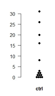
# Plotting original data as dots : first download the function plotdot in the file plotdot.R and data set data4samples.xls
# With the plotdot function executed in your session, here are two examples,

# first with a single sample (the control sample), then with multiple samples.

# After plotting, adjust window size so the dots are spaced out as desired
ctrl <- c(1,0,1,2,2,8,16,31,0,0,20,0,26,1,3)

plotdot(ctrl, names="ctrl", cols="black", pch=19, ypos=0.5)
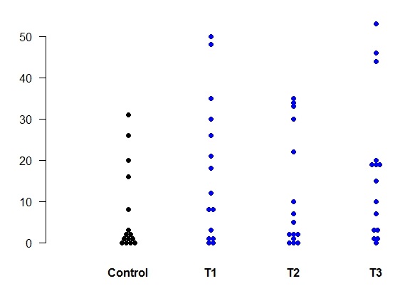
# Read in the data from the Excel file data4samples.xls into the matrix 'data' and then do the plot

# To make sure it's a matrix, perform the as.matrix function first.
data <- as.matrix(data)

plotdot(data, pch=rep(19,4), cols=c("black","blue","blue","blue"))
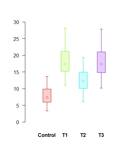
# Univariate confidence plots of the four samples in the data set data4samples.xls using function CIplot_uni (download it)
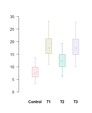
# Read in the data from the Excel file data4samples.xls into the matrix 'data' and then do the plot

# To make sure it's a matrix, perform the as.matrix function first.

# The default colours are the rainbow colours in R, some stand out more than others.

# The second plot shows a more even colour scheme using HCL palette in package colorspace
data <- as.matrix(data)

CIplot_uni(data, shade=T, ylim=c(0,30), thin=1.5)

require(colorspace)

CIplot_uni(data, shade=T, ylim=c(0,30), thin=1.5, cols=rainbow_hcl(4))
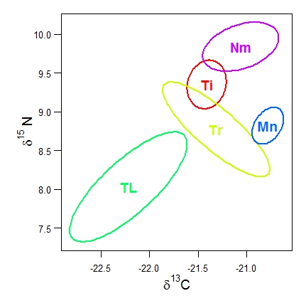
# Bivariate confidence plots of the istope data in the data set data2isotopes.xls using function CIplot_biv (download it). The ellipse package in R should be installed.
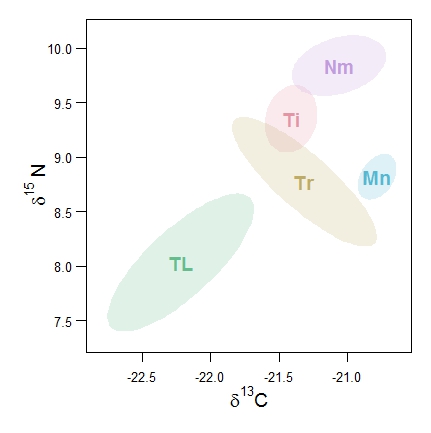
# Read in the data from the Excel file data2isotopes.xls into the matrix 'iso'

# Here it is supposed that the two isotope variables are in columns 2 and 3 of iso and the species codes/names are in column 1

# The first plot uses default ellipses based on the bivariate normal distribution, and default rainbow colours.

# The second plot uses bootstrap confidence ellipses, the HCL colours as well as shading.

# I also show how to label the axes with delta notation in R.
require(ellipse)

CIplot_biv(iso[,2], iso[,3], group=iso[,1], varnames=c(expression(paste(delta^13, "C")),

                expression(paste(delta^15, " N"))), lwd=3, cex=1.5,

                groupnames=c("Ti","Tr","TL","Mn","Nm"))

require(colorspace)

CIplot_biv(iso[,2], iso[,3], group=iso[,1], varnames=c(expression(paste(delta^13, "C")),

                expression(paste(delta^15, " N"))), ellipse=1, groupcols=rainbow_hcl(5), lwd=3, cex=1.5,

                groupnames=c("Ti","Tr","TL","Mn","Nm"), shade=T)